


Overview :
In this article, we will be making a project on, how to analyze and predict, the upcoming prices of Gold, using Machine Learning’s Random Forest Regressor. Sounds fascinating? Let us get on with it then..!!
Random Forest Regression in Brief
To understand what Random Forest Regression Algorithm is, a simple yet crisp definition will be, “Random Forest Regression is a supervised learning algorithm that uses ensemble learning method for regression. It operates by constructing several decision trees during training time and outputting the mean of the classes as the prediction of all the trees“, as stated in the levelup.gitconnected’s article.
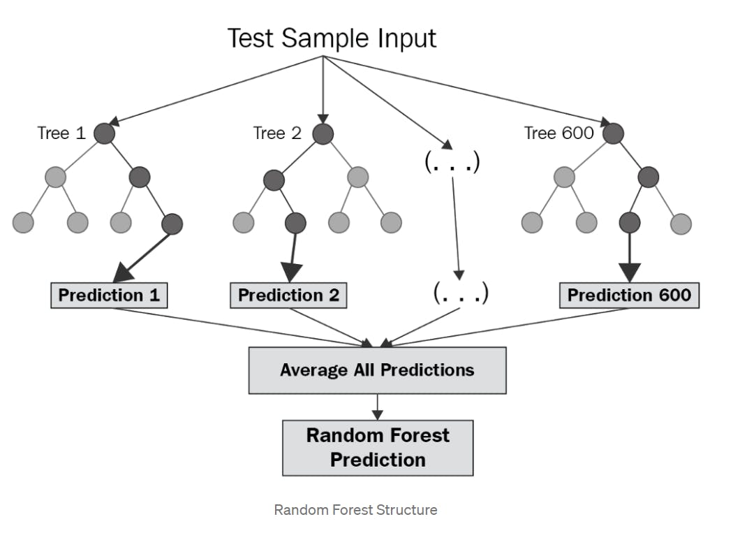
Image source : link
Building Our Project:
Note : This youtube video inspires this Project. Make sure to check it out too after reading this article: link.
For a better understanding of what are we going to do in this project, let us refer to a workflow to know our plan.
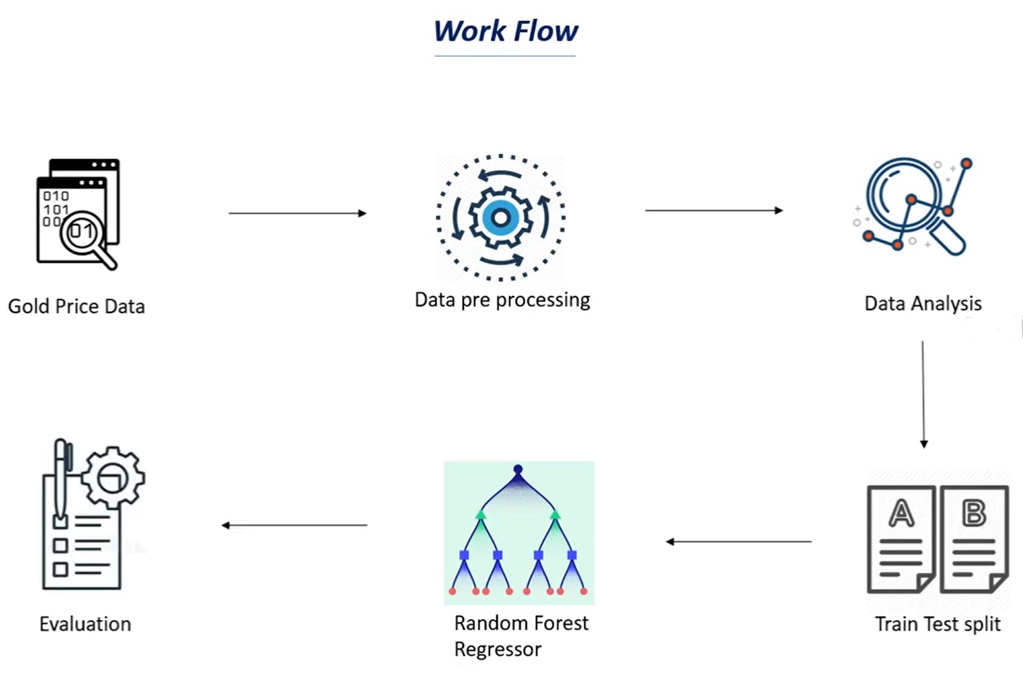
As we are now aware of what lies ahead, to accomplish this task, we shall begin with the very first and the most important thing needed in machine learning, a Dataset.
Dataset Description :
In this project, I have used the dataset available on Kaggle. One can find various such sites to download from. (Note that the larger the dataset, the more time the model will take to train. As a beginner-friendly suggestion, I will tell you to take a medium-sized dataset with not too many values, to first understand its working.)
The dataset that I used in my code was the data available on Kaggle. You can also download it from the link here.
Although, you must also know, the more data you feed to the model for training, the more we can train our model, and the more accurate our results come out to be, but also, at the same time, the compilation time increases, and if you are a beginner, you may lose your enthusiasm in that tedious times. Don’t worry if all of this sounds weird to you, it did the same to me when I started too, it will all make sense in a few minutes :)
Coding The Project :
As we will be using python for this project, we will also be needing a suitable environment for our code to run. You can use any environment that you prefer (E.g. Pycharm, VS Code, Sublime, etc.). In my case, I’ve used Google Collaboratory, as it removes the tedious process of compilation in the computer itself, and any type of code can be run very easily.
Dependencies:
The first thing that we have to do, is we have to import the necessary dependencies, that we will be using in the upcoming part of the program. Here in this project, we shall be using numpy, pandas, matplotlib, sklearn.
import numpy as np
import pandas as pd
import matplotlib.pyplot as plt
import seaborn as sns
from sklearn.model_selection import train_test_split
from sklearn.ensemble import RandomForestRegressor
from sklearn import metrics
As we proceed with our project, you will get to know the use of each of these modules. All you need for using Google Colab is a stable internet connection.
Reading The Dataset:
As the dataset file downloaded, is in the form of a CSV file, to read it, we will be needing the pandas module. It comes with a method read.csv() to read CSV files.
Let’s store it in a variable named ‘gold_data‘
gold_data = pd.read_csv('/content/gold price dataset.csv')
To get a look at how the data was stored in the variable, we use the command variable_name.head(), to see the first five rows of the table.
gold_data.head()
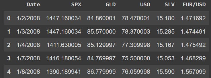
The above is the output.
The meaning of the Column values (SPX, USO, etc.) can be found on the website from which we have downloaded the dataset.
We saw on Kaggle while downloading the data set, that the data has 2290 rows and 6 columns.
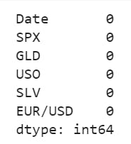
Now, let’s check how many cells are left empty in the table, to get a better insight :
gold_data.isnull().sum()
The output was :
Splitting Data into Target and Features:
X = gold_data.drop(['Date','GLD'],axis=1)
Y = gold_data['GLD']
As there were no empty cells, we could readily begin with the table manipulations;
Here, X is the feature variable, containing all the features like SPX, USO, SLV, etc., on which the price of gold depends, excluding the GLD and Date column itself.
Y, on the other hand, is the target variable, as that is the result that we want to determine,i.e, the price of Gold. (It contains only the GLD column).
Splitting Dataset into Testing Sets and Training Sets:
X_train, X_test, Y_train, Y_test = train_test_split(X, Y, test_size = 0.2, random_state=2)
Let’s understand the variables by knowing what type of values they store :
X_train: contains a random set of values from variable ‘ X ‘
Y_train: contains the output (the price of Gold) of the corresponding value of X_train.
X_test: contains a random set of values from variable ‘ X ‘, excluding the ones from X_train( as they are already taken).
Y_test: contains the output (the price of Gold) of the corresponding value of X_test.
test_size: represents the ratio of how the data is distributed among X_trai and X_test (Here 0.2 means that the data will be segregated in the X_train and X_test variables in an 80:20 ratio). You can use any value you want. A value < 0.3 is preferred.
Model Specification and Definition:
We shall be using a Random Forest regressor model.
We name our model ‘regressor‘.
regressor = RandomForestRegressor(n_estimators=100)
Now let us train the model, with our values containing the training dataset which are(X_train, Y_train)
regressor.fit(X_train,Y_train)
The model trains in a way like this: “When the values of X are these, then the value of Y is this.”
Evaluating The Defined Model :
Let’s now predict the values of the X_test dataset using the predict() method to test the accuracy of the model.
test_data_prediction = regressor.predict(X_test)
Calculating the R-Squared error from the predicted value :
error_score = metrics.r2_score(Y_test, test_data_prediction)
print("R squared error : ", error_score)
The output comes out to be: “R squared error: 0.9887338861925125”, which is an excellent score..!!
Comparison of Actual vs Predicted values :
Converting the values of Y_test into a list.
Y_test = list(Y_test)
Now, plotting values of actual prices, versus the predicted prices to know, how close our predictions were to the actual prices :
plt.plot(Y_test, color='blue', label = 'Actual Value')
plt.plot(test_data_prediction, color='green', label='Predicted Value')
plt.title('Actual Price vs Predicted Price')
plt.xlabel('Number of values')
plt.ylabel('GLD Price')
plt.legend()
plt.show()
And the output came out to be :
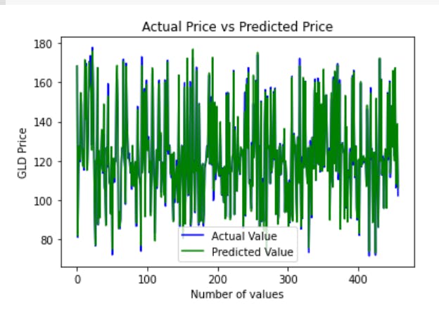
Thus we can observe, that the actual prices and the predicted prices are almost the same, as the two graphs overlap each other. Thus, our model has performed extremely well..!!! Congrats..!!
Parting Notes:
As you saw in this project, we first train a machine learning model, then use the trained model for prediction. Similarly, any model can be made much more precise, by feeding a very large dataset, to get a very accurate score (but it will be pretty time-consuming). For a beginner, I feel the dataset that I used was pretty decent.
Thanks for reading…
If you liked the article, do share it with your friends too.
Have a good day..!!
Please feel free to connect with me through my socials. I always love to have a chat with similarly-minded people.